Modelling survival in old age: Beyond proportions and cross-classification

Said Shahtahmasebi, PhD

The Good Life Research Centre Trust, Christchurch, New Zealand.

Correspondence: email: radisolevoo@gmail.com

Key words: binary, statistical modelling, longevity

Received: 15/10/2019; revised 15/11/2019; Accepted: 25/11/2019

[citation: Shahtahmasebi, S. (2019). Modelling survival in old age: Beyond proportions and cross-classification: DHH; 6(4):http://www.journalofhealth.co.nz/?page_id=1940].

Introduction

The North Wales Elderly Project (NWEP) was a longitudinal study of old age in rural North Wales (UK), see (Wenger, 1984). A large social survey of a sample of randomly selected elderly people in North Wales was carried out in 1979. In 1983 and 1987 the sample members were traced, their status (e.g. whether alive or deceased) was recorded, and the survivors were surveyed using the same questionnaire. Subsequent surveys during the 1990s mainly traced and surveyed the sample members with a much shorter version of the questionnaire. The purpose of this study was to investigate the support network and coping dynamics of elderly people living in rural areas. The study provided rich three-time point information on the sample of elderly people including individual characteristics, support network, health and dependency, quality of life, perceptions and expectations. Included in the strategy for analysing of longitudinal social survey data, which is reported elsewhere (Shahtahmasebi & Berridge, 2010) was to address the question ‘what factors govern survival in old age?’

The analysis of survival is exploratory for three main reasons. Firstly, the relationship between social circumstances and longevity is a speculative area lacking the theoretical and empirical foundations necessary for the design of a sharply focused study. Even the effect of social class on survival is uncertain for the elderly, with several studies (Fox & Goldblatt, 1982; Reid, 1977; Townsend & Davidson, 1982) suggesting that the class effect evident for younger age groups tends to tail off by the age of retirement, while others (Phillipson, 1982; Victor & Evandrou, 1986) suggest that the variations due to social class in early life are carried through into old age. Secondly, the high multicollinearities between many variables and the possibly complex causal relationships involved make it difficult to disentangle the different effects compounded in the data. In particular, data from regular re-interviewing would be necessary to identify how different health, dependency, and social factors interact over time in whatever impact they have on short and long-term survival. Finally, inference is limited by a sample selection bias effect (Lancaster & Nickell, 1980; Vaupel, Manton, & Stallard, 1979). The problem is that everyone in the sample has, of course, survived to the date of the first interview. As the more frail will not have survived, many of the older individuals in the sample will be inherently stronger than might be expected given their observed characteristics. This will attenuate the effect of the observed characteristics in any statistical analysis of subsequent survival; systematic effects will be more difficult to detect. The problem is exacerbated by the fact that the sample excludes those in residential care at the time of the original survey.

The literature suggests a number of socio-economic, biological and individual characteristics to be associated with survival. For example, higher levels of occupation and class, income, and/or education as indicators of socio-economic status appear to be associated with lower morbidity and mortality. Conversely, bereavement (usually, widowhood) (Jagger & Sutton, 1991; Jones, 1987; Thompson, Breckenridge, Gallagher, & Peterson, 1984), no supportive network and social isolation (Berkman & Syme, 1979; Kaplan & Camacho, 1983) are reported to be associated with higher morbidity and mortality rates.

One of the contending issues is that these results are mainly based on cross-tabulation of data which explores the relationship between two variables. Cross-classification of data does not allow accounting for other variables when exploring the effect of an explanatory variable on the outcome variable (in this case survival in old age). For example, social factors’ effects on longevity may be in part through age and sex effect. Therefore, age and sex must be accounted for when investigating the net effect of a social factor.

In this article, using a secondary data source, survival in old age is explored using statistical modelling that allows additional control in the analysis over and beyond cross-classification technique.

Data

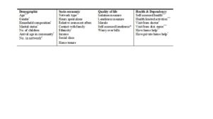
Variables of interest, including demographic, socio-economic, quality of life, and health and dependency were extracted from the NWEP. The availability of data on such a large number of variables presented a unique opportunity to investigate relationships with survival four years (1979-1983–1987) and eight years (1979-87) later.

There were a number of ways of analysing survival data provided by NWEP e.g. see (Shahtahmasebi, Davies, & Wenger, 1992). The simplest way to create a survival response is obviously to create a dummy variable containing all the respondents who had survived until the tracing interval as alive (or success) and the non-survivors as deceased (or failure), and drop those cases which could not be traced and where there was no information on them (missing cases) from the analysis.

Social circumstances were defined very broadly, covering social class, other socio-economic and social characteristics, quality-of-life, level of dependency, and perceptions of health.

Missing values

Less than one percent of the cases had missing values for most variables. The simple “imputation” strategy of allocating such cases to the variable categories with the highest frequency was adopted. However, there were rather more missing observations for the variables income, number in network, morale, isolation measure, and loneliness measure. For income, fieldwork experience indicated that the majority of refusals were from higher income respondents and all were allocated to the upper income category. A separate non-response category was retained for the remaining variables.

Data limitations

Data limitations also prevent from proceeding to investigate the effect of interactions between variables; the frequencies in subcategories became too small for reliable analysis. Not unreasonably for an exploratory study, the focus was solely upon the “main effects” of the explanatory variables. Besides, the hierarchy principle (Bishop et al 1988) suggests that interaction terms should be included in the model only when the relevant main effects are also present in the model.

Bivariate analysis

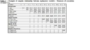
Simple cross-classifications confirm that most of the explanatory variables were significantly related to survival over the eight year period 1979-1987. This information is summarised in Table 1. About 62% of the variables were significant at the 5% level. In addition three more variables were significant at the 10% level: “social class” (p=0.094), “morale” (p=0.07), and “loneliness measure” (p=0.09). It is quite plausible that some of these effects owe their significance to their association with age. Moreover, Cramer’s υ measures of association (Table 2) confirm that there are complex patterns of inter-relationships between the explanatory variables and that it would therefore be unwise to attempt any direct interpretation of these bivariate cross-classifications with survival. Thus, for example, Cramer’s υ indicates that network type varies with age and several of the dependency and health variables. Network type proved to be highly significant (Table 1) but does this reflect a social determinant of survival in old age or is network type merely acting as a proxy for age, dependency, or health effects? A multivariate analysis is therefore required to enable ceteris paribus conclusions about the effects of each explanatory variable on survival.

 

Table 1 – Bi-variate cross-classification of survival/non-survival with some explanatory variables (% survived in each category)(goodness of fit is based on the Pearson χ², *£0.05, **£0.01, ***£0.001) – N=524.

 

Statistical modelling

We are interested in the net effect of explanatory variables on survival in old age. In examining the net effect of an explanatory variable on the response we must account or “control” for the effect of other explanatory variables.

One way of introducing “control” in the analysis is the method of disaggregation i.e. multi-way Tables cross-referencing the response with an explanatory variable for a selected category of another explanatory variable. There were several problems with such an approach. Firstly, it is an extension of the cross-classification process and will lead to numerous Tables to examine and interpret. In studies of this type where a large number of variables are involved, examination and interpretation of a large number of Tables will be cumbersome, painstaking and speculative, and may lead to unsatisfactory results. Secondly, multi-way cross-referencing may lead to (very) small cell frequencies which cannot be interpreted in a meaningful way. Thirdly, this method gives a jagged picture of the data because it will not allow the smoothing out of continuous variables e.g. age will have to be categorised. Furthermore, it provides no facilities to quantify and compare the prevalence for a given group with that of a reference group.

Analysis

The analysis seeked to explore the pattern of association between explanatory variables and survival eight years on at the end of the project “window”. The tracing variables at 1983 and 1987 provided survival outcomes e.g. alive and in community, alive in residential care, deceased, as well as duration survived. A number of analyses were possible such as binary response (alive/deceased), multinomial (alive, in care, deceased), and duration dependence (length of time survived), e.g. see (Shahtahmasebi & Berridge, 2010; Shahtahmasebi et al., 1992).

This article presents the analysis of the simple case of a binary outcome of survived to 1987 (1), or deceased at 1987 (0).

In general, the logistic regression model is an appropriate model to fit to data when the outcome is a binary variable, e.g. success or failure, yes or no (0, or 1). This model can be fitted in most statistical packages. The model selection and criticism was based on the log-likelihood test statistic (χ²).

Modelling process

Because of the large number of variables, a “forward” iterative method of selection was adopted. Variables were entered in the model one at a time. The best model was selected based on their contribution to the likelihood function, and those variables which are not significant at 5% level were dropped from the analysis. Model selection is repeated with the remaining variables using the selected best model until there are no variables remaining significant at the 5% level. This approach can be very instructive in an exploratory study. In particular, a marked change in the significance of a remaining variable when a new variable is added to the model is indicative of a spurious relationship arising from statistical association with the added variable. On the other hand, with high multicollinearity in the data, the final model may be heavily dependent upon a marginal choice between two variables at some stage in the model fitting process. It is important to detect when this is occurring to prevent undue emphasis being given to one variable where others are practically indistinguishable in their explanatory power. Moreover, identification of nearly interchangeable variables may guide further research in reducing multicollinearity problems by combining variables in composite indices.

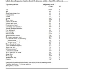
As shown in Table 3 there are 18 variables which appear to be significantly related to survival without any control. Once age, sex and self-assessed health are entered in the model there are only 6 variables which remain statistically significant. Out of these only the variables ‘arrival age’, ‘visits from district nurse’ and ‘ethnicity’ were accepted in the final model for the base-line data. The model fitting results are shown in Table 4.

A specific example of multicollinearity is provided by the variables “self-assessed health” and “health limited activities”. These two variables appear to be significantly related to survival on their own (single model; χ²₁=33.0 and χ²₂=15.9). However, when controlling for “age” and “self-assessed health”, “health limited activities” ceases to be significant (χ²₂=0.1). In this instance, the inclusion of “health limited activities” does not add anything to the results over and above age and state of health.

In practice, when selecting a model, it is not uncommon to encounter an ambiguity problem. This means situations where after fitting models the resulting p-values for the effect of two explanatory variables are very small or sufficiently close that we are unable to distinguish a dominant effect. Under such circumstances alternative models should be constructed which may lead to the examination and the interpretation of more than one parsimonious model.

Interpretation

As noted earlier, the statistical modelling approach resulted in reducing the number of variables which appear to be statistically associated with survival/non-survival to 6 (out of those present in Table 1). Some of those variables which were significant at 5% level when on their own, such as marital status, house tenure (see Table 3) are no longer significant. It seems that when controlling for age the significance of these effects is reduced considerably, and when controlling for both age and sex, the inclusion of house-tenure-effect and marital-status-effect in the model add nothing further to the results.

While this analysis focuses mainly on the variations due to main effects, it is possible to introduce and test for interaction effects even at a late stage when the parsimonious model(s) has been accepted. This can be done by creating a dummy variable representing the interaction effect of interest in the final model, e.g. a dummy variable may take values of 1 for “male and widowed”, and 0 for “other”.

To fully explore the effect of each variable on the model of survival, alternative restricted models were compared with the full model. This was done by dropping an explanatory variable from the full model, observing the change in the model and then replacing it back into the model. This process was repeated for all the variables which are in the full model. The full model fitting results are shown in Table 4, which also show the likelihood ratio (χ²) for each restricted model and their respective associated p-value. A further feature of this method is the facility to calculate the survival probabilities (alternatively odds ratios could easily be calculated and used) for each explanatory variable other things being equal, see appendix.

As expected, age and sex are strongly related to survival; increasing age decreases the probability of survival and women live longer. Probability of death given a female respondent is shown to be 0.23 (Table 4), a small probability, indicating higher chances of survival (other characteristics being the same). Similarly, a poor state of health increases the probability of death in old age (other characteristics being the same). It seems that “visits from district nurse” variable “mops up” some of the variation in survival rate due to frailty (ill-health) but left unexplained by the self-assessed health variable.

There is sufficient evidence (p=0.025, Table 4) to suggest that visits from the district nurse are significantly related to non-survival. A direct translation of the parameter estimates should not be taken to indicate that regular or increased visits from the district nurse would increase the likelihood of death! The data and frequency distribution of visits from the district nurse showed that those who were more dependent and/or in ill health were more likely to receive visits from the district nurse. This is a causality problem where an impending event causes a reaction, i.e. the impending death causes visits from the district nurse. Indeed, visits from the district nurse became more likely and frequent in the weeks/months preceding death. Clearly the state of health variable does not fully control for this effect. Visits from the district nurse may also be related to the frailty of advanced old age and the need for help with bathing, not necessarily associated with ill health.

Note that in Table 4 “ethnicity” is included in the model marginally at the 5% level. It can be seen that the significance of this variable is mainly due to the large effect from those who classified themselves as “British”. Interrogation of the data suggested that this may be reflecting an interaction with social class; those in this category appear mostly to be of middle class background.

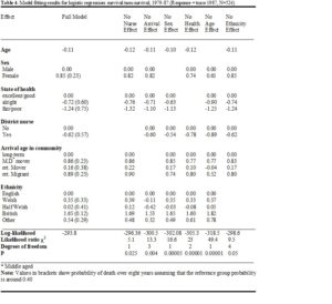
There is sufficient evidence that the variable ‘arrival age’ is related to survival (p=0.004). The results in Table 4 appear to suggest that those who have moved more than 25 miles after age of 60 (middle aged movers, and retired migrants) have a higher likelihood of survival than long-term residents. In contrast those who moved short distances after the age of 60 (retired movers) appears to be no different to the reference group (long-term residents). The variable ‘arrival age in the community’ (Table 4) can reflect availability of kin and the likelihood of being alone. Those who arrived in the community before or during child-rearing age were more likely to have local kin networks than those who arrived in middle or old age. Thus, those who have lived for many years in the same community had more access to kin in the face of growing dependency. Support networks were shown to be relatively stable in the long term (Wenger & Shahtahmasebi, 1990). Well established, long-term residents might be expected to live longer. The above results suggested the opposite. The association of this variable and social class (p=0.0003) may well explain, at least in part, these counter intuitive results. It appears that the movement of those in lower social class groups takes place mainly within the community. On the other hand, the long-term residents were more likely to have had a well-established support network which while it may not increase longevity it will increase the level of support and care needed due to dependency in ill health, old age and frailty.

An important result from these analyses is that none of the quality of life variables in the data appeared to be related to survival (e.g. morale, loneliness). Inclusion of age and sex in the model appears to control for the effect of quality of life variables as none remained significant. In the context of survival the variables ‘arrival age in community’, ‘self-assessed health’ and ‘ethnicity’ tend to reflect dependency due to ill-health.

Summary and conclusion

A bi-variate cross-classification of survival/non-survival with a list of explanatory variables was presented in Table 1. It was illustrated that cross-referencing is simple and easy to carry out with measures (e.g. χ²) of the strength of the relationship (e.g. using SPSS). Although, bi-variate cross-classification is a useful step in getting an idea about the data, however, if taken as independent inferential statements is of meagre value (Berridge, 2014). This is due to the lack of any control when investigating the relationship between the response and explanatory variables (also see (Berridge, 2014)).

This article, thus, demonstrated the application of statistical modelling to disentangle the complex relationships among the variables. This enabled:-

• The exploration of the relationships between survival and each explanatory variable in the presence of other variables, i.e. control for other effects, thus identifying systematic effects,
• The exploration of the relationships between explanatory variables (multicollinearity), e.g. relationships between age, sex, self-assessed health and health limited activities,
• The estimation and quantification of the effect of explanatory variables on survival in terms of probabilities enabling conclusions about the effect of each explanatory variable on survival other characteristics being the same,
• Finally, with the application of statistical modelling the large number of variables thought to be related to survival was reduced to a few variables which are easy to manage and interpret.

 References

Berkman, L. F., & Syme, S. L. (1979). Social Networks, Host Resistance, and Mortality  A Nine-Year Follow-up Study of Alameda County Residents. American Journal of Epidemiology, 109, 186-204.

Berridge, D. (2014). Paper 3.  The Exploratory Analysis of Data on Survival in Old Age. Dynamics of Human HEalth (DHH), 6(1), http://www.journalofhealth.co.nz/?page_id=1752.

Fox, A. J., & Goldblatt, P. O. (1982). Longitudinal study  socio-demographic mortality defferentials. London: OPCS, HMSO.

Jagger, C., & Sutton, C. J. (1991). Death after bereavement – Is the risk increased? Statistics in Medicine, 10, 395-404.

Jones, D. R. (1987). Heart Disease Morality Following Widowhood: Some Results From the OPCS Longitudinal Study. Journal of Psychosomatic Research, 313, 325-333.

Kaplan, G. A., & Camacho, T. (1983). Perceived Health and Mortality: A Nine year Follow- up of the Human Population Laboratory Cohort. American Journal of Epidemiology, 117, 292-304.

Lancaster, T., & Nickell, S. (1980). The analysis of re-employment probabilities for the unemployed. Journal of the Royal Statistical Association, Series A; 14@3, 141- 165.

Phillipson, C. (1982). Capitalism and the Social Construction of Old Age. London: Macmillan.

Reid, I. (1977). Social Class Differences in Britain. London: Fontana.

Shahtahmasebi, S., & Berridge, D. (2010). Conceptualising behaviour in health and social research: a practical guide to data analysis. New York: Nova Sci.

Shahtahmasebi, S., Davies, R., & Wenger, C. (1992). A longitudinal analysis of factors related to survival in old age. The Gerontologist, 333, 404-413.

Thompson, L. W., Breckenridge, J. N., Gallagher, D., & Peterson, J. (1984). Effects of Bereavement on Self-Perceptions of Physical Health in Elderly Widows and Widowers. J. of Gerontology, 393, 309-314.

Townsend, P., & Davidson, N. (1982). Inequalities in Health – The Black Report. Suffolk: The Chaucer Press.

Vaupel, J. W., Manton, K. G., & Stallard, E. (1979). The Impact of Heterogeneity in Individual Frailty on the Dynamics of Mortality. Demography, 163, 439-454.

Victor, C. R., & Evandrou, M. (1986). Does Social Class Matter in Later Life? In S. Gregorio (Ed.), Social Gerontology: new directions. London: Croom Helm.

Wenger, G. C. (1984). The Supportive Network – coping with old age. London: George Allen and Unwin.

Wenger, G. C., & Shahtahmasebi, S. (1990). Ageing and dependency in rural areas: eight years of domiciliary visiting of old elderly. CSPRD, University of Bangor, Gwynedd, U.K.