Modelling Survival in Old Age: Duration Dependence

Said Shahtahmasebi, PhD

The Good Life Research Centre Trust, Christchurch, New Zealand.

Correspondence: email: radisolevoo@gmail.com

Key words: duration, statistical modelling, longevity

Received: 2/2/2020; revised 5/3/2020; Accepted: 25/3/2020

[citation: Shahtahmasebi, S. (2020). Modelling Survival in Old Age: Duration Dependence. DHH, 7(2):http://www.journalofhealth.co.nz/?page_id=2166].

Introduction

As reported in the first paper on survival in old age the data came from a large social survey study of elderly people living in rural North Wales (NWEP), UK, which followed a randomly selected sample of elderly households at four-years interval in 1979 (Wenger, 1984). The full range of longitudinal strategy for analysis is reported elsewhere (Shahtahmasebi & Berridge, 2010). The purpose of these three papers is to demonstrate gained insight into survival through increased complexity in the analysis due to the provision of additional information.

The binary and multinomial models that were employed to analyse survival data reported in the last two issues of DHH use only partial information i.e. whether an observed case is alive, in care or deceased. An individual whose status in 1987 was recorded as deceased could have died at any point in time during the study window 1979-87. The individual may have died just after the 1979 interview or may have died just before the 1987 interviews; these are two very different outcomes. This level of information is lost in the logistic regression models presented in the previous two papers (Shahtahmasebi, 2019, 2020). In particular, date of death is needed to account for the duration survived in the project window. To fully utilise time survived the application of a more complex model is essential.

Statistical Modelling of Survival Times

Here, survival time refers to the actual length of time an individual survived. Since all individuals were alive and in the community at the start of the project, the maximum survival time is equal to the length of the 1979-87 study ‘window’ with October 1987 being the cut-off point i.e. 8.5 years. The data are right censored. This means that all the individuals who were alive by the cut-off point will be assigned the maximum survival time of 8.5 years. Therefore, all sample members will have an observed duration (T). Unlike the binary and multinomial analysis in which the outcome is categorical duration survived is a continuous variable so the logistic model is not appropriate for continuous outcome variables. This type of data can be modelled routinely using the Weibull model as briefly described in the appendix.

The NWEP was designed primarily to explore how elderly people live in rural areas. As such, the main interests related to the elderly people’s social networks, sources of care and support, wellbeing and physical health, involvement in the community and access to amenities.

A substantive issue arises. Social circumstances will have an impact on survival, in part, by affecting health and, possibly, dependency. Controlling for these variables may therefore result in an over-conservative, attenuated estimate of the effects of social circumstances. Reverse causality is also possible, with health and dependency influencing social circumstances. Excluding these factors may therefore exaggerate the effects of social circumstances. Therefore, a pragmatic approach to this problem was to repeat each analysis with and without the health and dependency variables.

The ‘forward substitution’ model fitting procedure was adopted. Briefly, variables were entered in the model one at a time with the ‘best’ additional variable added to the model at each stage. The improvement in the model as a result of adding each variable in turn was assessed by a likelihood ratio test statistic and the process ceased when no additional variable was significant at the 5% level. Out of 30 explanatory variables only 5 remained significant at %5 and selected into the model. The results from the model fitting process are shown in table 1.

The substantive issue mentioned above is tackled by repeating the model fitting without the health and dependency variables. No additional social variables were included in the model. The results are shown in Table 1; the values in parentheses are the results when the health and dependency variables were excluded from the model. It can be seen that the changes in the parameter estimates for the remaining variables were modest. The health variable and dependency measures do not appear to be important control variables when examining the relationship between social characteristics and survival.

Interpretation

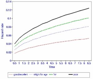
It is clear that the elderly people’s subjective assessment of their own health has high predictive value for subsequent survival. The inclusion of the ‘district nurse’ variable in the main model warns us that this subjective assessment is not a fully effective measure of ill-health, dependency and other aspects of frailty. However, self-assessed health is decidedly superior to the other indicator variables considered. From Table 1, the elderly assessing their health as ‘all right for age’ have about 1.5 times the death rate of those with excellent/good health. The figures for fair and poor self-assessed health are about 2 times and 2.4 times respectively. These results can be seen more clearly diagrammatically, by plotting the hazard rate for given values of the explanatory variable over time. For example, Figure 1 illustrates how the risk of dying over time varies from one category of (self-assessed) health to another. The hazard rate rises more steeply for elderly individuals who assessed their own health as poor than for those who assessed their health as good/excellent (other characteristics being the same: aged 65, male, owner occupier, who did not receive visits from a district nurse). It can be seen that the hazard rate for those in good/excellent health is much flatter than the hazard rates for those in other categories of self-assessed health, which rise more sharply and maintain an upward trend over time.

Table 1. Model fitting results controlling for duration dependence, N=524

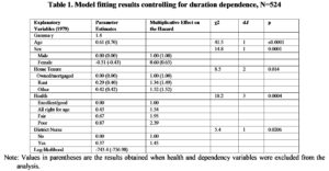
Note: Values in parentheses are the results obtained when health and dependency variables were excluded from the analysis.

The socio-economic variable ‘home tenure’ appears to be related to mortality in old age. From Table 1, the elderly in rented accommodation have about 1.3 times, and those in the ‘other’ category (including living with relatives other than spouses) have about 1.5 times the death rate of owner occupiers, other characteristics being equal. It is noted that these figures may include some element of dependency over and above that represented by the other variables in the model. For example, those living with relatives may tend to be more frail. Nevertheless, the significance of the ‘home tenure’ variable suggests that survival is affected by socio-economic factors which are not adequately represented by the social class and income variables.

Figure 1. Diagrammatical illustration of how hazard rates vary by (self-assessed) health.

Summary

To examine how the different models of survival performed the results for the three models is summarise in Table 2. Generally, the results from the binomial, multinomial and hazard models appear consistent. In particular, none of the results suggests any quality of life effect on survival, even when excluding the health and dependency variables from the model. The subjective assessment of dependency as measured by the variable ‘state of health’ appears to be a better predictor of survival than any other objective measures of dependency that were included in the analysis.

The multinomial model appears to agree with the hazard and binomial logistic models on the demographic variables age and sex. Furthermore, they also agree on the same measure for morbidity ‘self-assessed health’. This variable appears to control fully for the effect of ill-health in the multinomial model i.e. it excludes the variable ‘visits from district nurse’. The models differ, however, in the choice of socio-economic variables. The binomial logistic model includes two socio-economic measures: ‘arrival age in community’ and ‘ethnicity’. The hazard and multinomial models each include one socio-economic measure: ‘home tenure’ and ‘arrival age in community’ respectively. Finally, it is emphasised that, with hazard modelling, we also obtain information about how mortality varies over time. This is illustrated in Figure 1.

Conclusions

With the cross-sectional modelling of survival, the multicollinearity issue was addressed. It was demonstrated that tackling this issue will help to reduce the number of explanatory variables thought to contribute to an outcome (survival in this case) to a manageable number. To some extent, accounting for multicollinearity also helped to explore and distinguish systematic effects in the data from random variations which tend to obscure any pattern. Advancing the analysis, from a standard logistic model to modelling multinomial response and duration survived, allowed us to take into account more information on individuals.

It is reasonable to assume that, when more information is included in the analysis, we may expect more informative results. However, this additional insight may be gained at a cost i.e. through increasing complexities in the model.

Table 2. Comparison of the three models fitted to the survival data

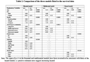
Note: The signs of p.e.’s in the binomial and multinomial models have been reversed to be consistent with those of the hazard model, i.e. positive estimates now suggest increasing hazard.

Briefly, it is clear that the ‘district nurse’ effect represents impending death and thus health and dependency. To some extent, the ‘arrival age in community’ effect also represents health and dependency; those who moved to the area early in life are more likely to have established social and care networks. On the other hand, the ‘arrival age in community’ effect is also a proxy for social class and income, as is ‘ethnicity’. The results from duration analysis (hazard model) suggest that the health and dependency variables directly influence survival over and above age and sex effect. However, the presence of ‘district nurse’ and to some extent ‘home tenure’ appear to ‘mop up’ some of the variation in survival rates due to frailty but had been left unexplained by the self-assessment variable. On the other hand, ‘home tenure’ may be a proxy for social class and socio-economic effects. However, the data suggest that those elderly people living in alternative accommodation, in particular with others, are more likely to be more dependent and less mobile.

In summary, the appropriate method of analysis is dependent on the type and nature of the response subject to relevant substantive issues. For example, when variables are collapsed into fewer categories we may inadvertently place dissimilar individuals into the same category. However, one has to be aware that (substantively viewed) this may not be as important an issue analytically. For instance, if we are primarily interested in the number of deceased then it may be reasonable to categorise all the deceased individuals into one category. When the interest lies in exploring the factors that may influence survival, then individuals who died at the start of the project window may well be different to those who died at the end of this period (in this example a difference in duration of 8.5 years). When grouped together, it is not possible to utilize fully the explanatory power of explanatory variables such as health and dependency. To some extent, we have got around the problem through collecting additional information e.g. for the survival example, we collected more data on the length of time an individual survived. The increased explanatory power in the statistical model we adopted comes from being able to account for each respondent’s contribution.

We were not able to use the dynamics of explanatory variables in these models, e.g. the true effects of ‘home tenure’ as an indicator of socio-economic effect or dependency, or change in health status from 1979 to 1983 and to 1987. These issues have been discussed previously, e.g. see (Shahtahmasebi & Berridge, 2010), and will be explored in the next issue of DHH in the context of morale in old age.

References

Aitkin, M., Anderson, D., Francis, B., & Hinde, J. (1989). Statistical modelling in GLIM. Oxford: Oxford University Press.

Cox, D. R., & Oakes, D. (1984). Analysis of Survival Data. New York: Chapman and Hall.

Kalbfleich, J. D., & Prentice, R. L. (1980). The Statistical Analysis of Failure Time Data. New York: Wiley.

Lawless, J. F. (1982). Statistical Models and Methods for Lifetime Data. New York: Wiley.

Shahtahmasebi, S. (2019). Modelling survival in old age: Beyond proportions and cross-classification. Dynamics of Human Health (DHH), 6(4), http://www.journalofhealth.co.nz/?page_id=1940.

Shahtahmasebi, S. (2020). Modelling Survival in Old Age: Multinomial outcome. Dynamics of Human Health (DHH), 7(1), http://www.journalofhealth.co.nz/?page_id=2057.

Shahtahmasebi, S., & Berridge, D. (2010). Conceptualising behaviour in health and social research: a practical guide to data analysis. New York: Nova Sci.

Wenger, G. C. (1984). The Supportive Network – coping with old age. London: George Allen and Unwin.

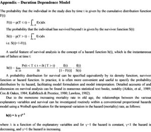
Appendix